The second part of our SoftGNSS series is about postProcessing and Acquisition. Post-processing is the general name for all progress after signal capturing, acquisition is the first step of the post-processing process.
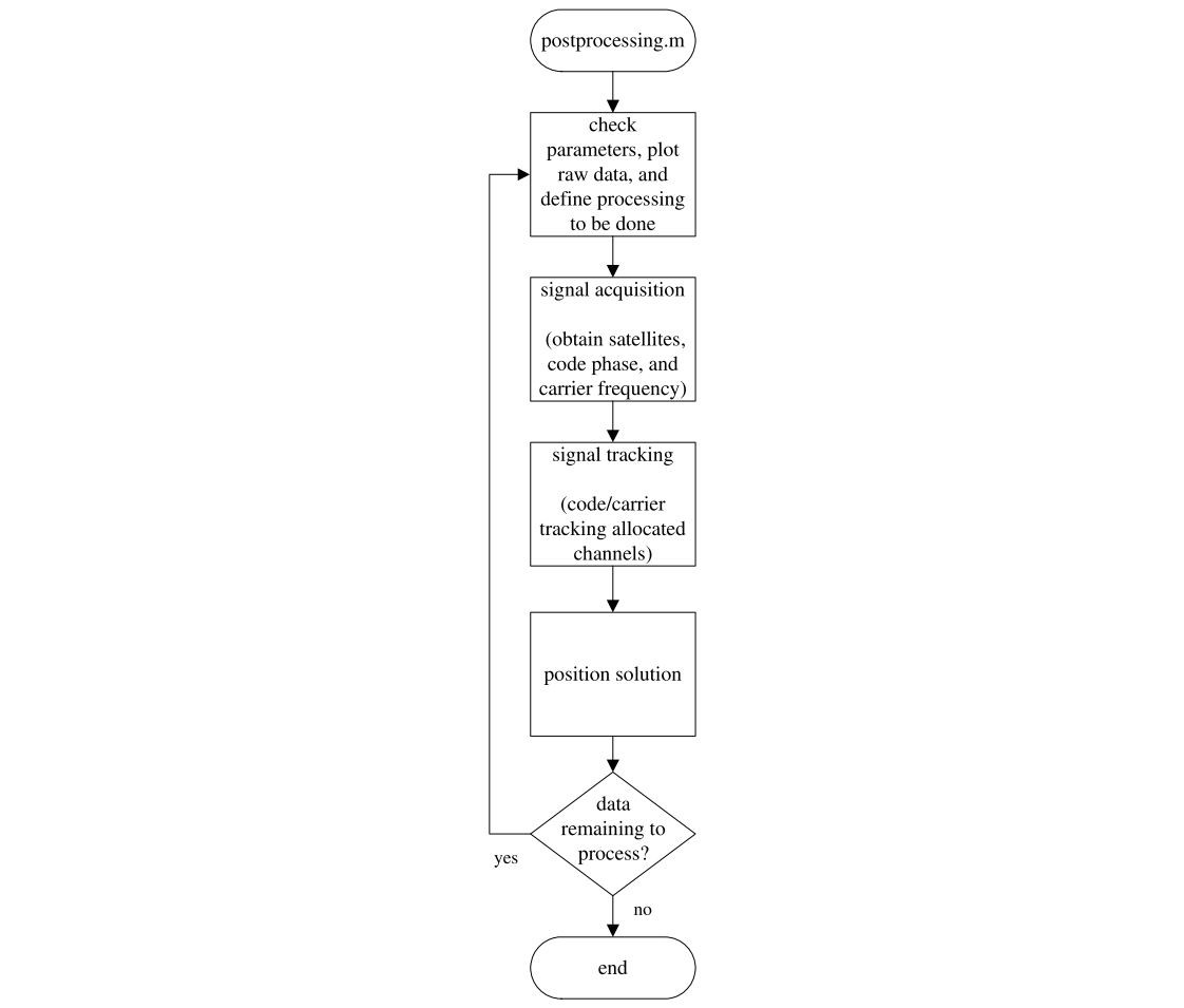
In the previous post, we focused on the first top square box in the diagram above, we called that process as probeData. Now we will focus on acquisition that is used to determine visible satellites and coarse values of carrier frequency and code phase of the satellite signals.
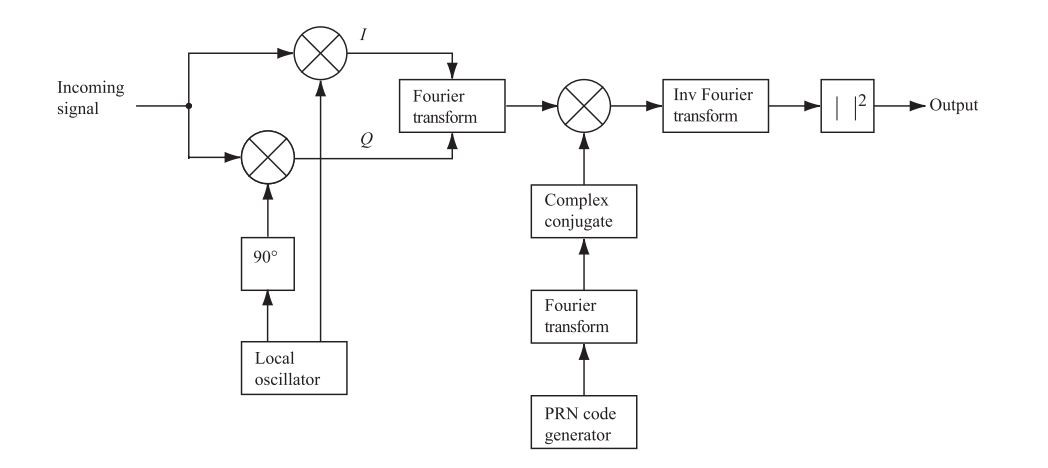
The code implies “Parallel Code Phase Search Acquisition” algorithm rather than other algorithms(Serial Search Acquisition, Parallel Frequency Space Search Acquisition) as mentioned in the book. Let’s analyze the algorithm first.
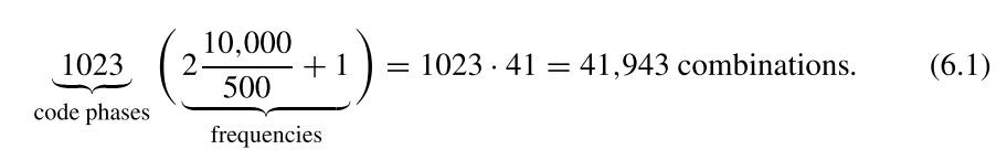
The bracket called frequencies above means +-10 kHz frequency changes by 500 Hz steps. The purpose of our algorithm is to reduce the number of combinations (41.943) above. So there are two parameters to reduce or remove: code phases and frequencies. The number of combinations above is produced by the multiplication of possibilities in the time domain. So we need to parallelize these processes using FFT or DFT. Working on the frequency domain for each parameter makes us faster so much.
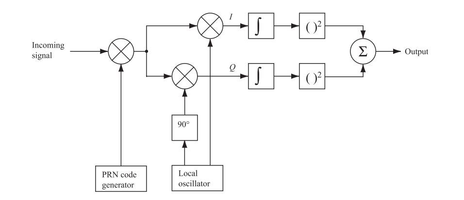
Our first parallelization method is about frequency space. Called “Parallel Frequency Space Search Acquisition“. In this method, the incoming signal is multiplied by code phases and the FFT analysis is done. So “frequency search” step is eliminated. The parallel frequency space search acquisition only steps through the 1023 different code phases.
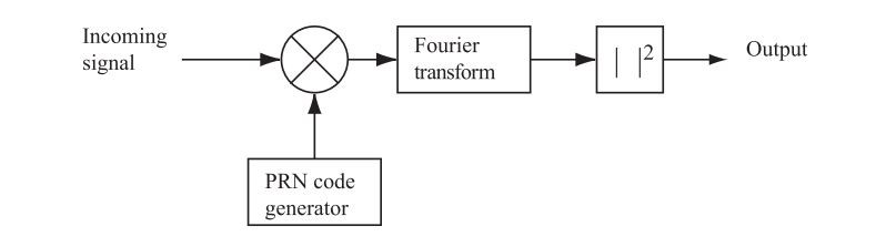
The second method is “Parallel Code Phase Search Acquisition“. The goal of this method is to perform multiplication with the incoming signal and a PRN code, instead of correlation in time domain. Compared to the previous acquisition methods, the parallel code phase search acquisition method has cut down search space to the 41 different carrier frequencies.
The execution time of the algorithms above is compared in the table below.
| Algorithm | Execution Time | Repetitions | Complexity |
| Serial Search | 87 | 41.943 | Low |
| Parallel Freq. Space Search | 10 | 1023 | Medium |
| Parallel Code Ph. Search | 1 | 41 | High |
Let’s analyze the implementation. As I have mentioned above, the code uses “Parallel Code Ph. Search” algorithm. The flow diagram of the code is drafted below.
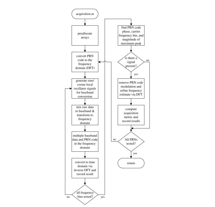
The first important point in the code we are focusing on is about creating two 1msec signals. The reason should be getting sure that the C/A signal what we are looking/wşill correlate is completely in it, getting two samples from the input signal which of length equals the C/A length, so we have 2msec signal. The C/A code repeats itself each 1msec so it can be found inside in any 2msec signal sample even if it is not aligned.
% Create two 1msec vectors of data to correlate with and one with zero DC
signal1 = longSignal(1 : samplesPerCode);
signal2 = longSignal(samplesPerCode+1 : 2*samplesPerCode);
The second main point is PRN iteration. It is a must as you know, all PRN codes have to be correlated if the signal contains any data on that PRN or not. PRN iteration contains another iteration called freqBin which uses for correlation for the whole freq band.
After each PRN iteration, we have a matrix called “results” containing the correlation of PRN and input signals with different frequencies based on freqBin variable (in our example, 29 different frequency shifting). After this step, you can manually find the acquisition result manually with a visual inspection. Below, I have an example for the inspection.
Let’s analyze two “results” matrices of two PRNs, one is acquiring; and the other is none. First PRN 1;
K>> subplot(2,1,1)
K>> plot(results(1,:))
K>> subplot(2,1,2)
K>> plot(results(20,:)) %20 has the max peak value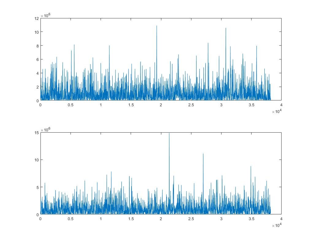
Now PRN 3;
K>> subplot(2,1,1)
K>> plot(results(1,:))
K>> subplot(2,1,2)
K>> plot(results(19,:)) %19 has the max peak value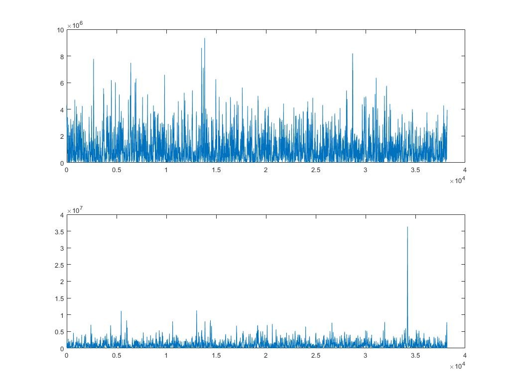
As you see clearly, the second graph of PRN 3 has a single high and peak value. So we can basically consider PRN 3 as acquired. However, to be sure that there are methods like comparing the highest peak with the second highest one, determining a threshold, etc.
The code we are using compares the highest peak with the second-highest peak; if the ratio is higher than the threshold, the PRN is added to the acquisition list. However, to get the PRN frequency value more accurate, the code uses additional steps for each acquired PRN.
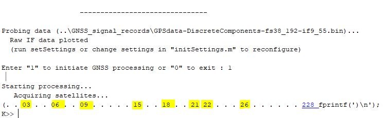
At the final of our “acquisition” function, we get the output below.
Leave a Reply