

Nowadays, I am studying BDS receiver. I found an open source B1C receiver, however it is not working what I expected. It needs to be improved maybe. Now, I am analysing it. The firs part I analysed is “acquisition” block/function.
While I was analyzing the function, I wonder the reason behind using FFT multiplication instead of time-domain correlation to find the delay value between two identical signals. And I researched it, here are a few explanations to read about it:
- https://en.wikipedia.org/wiki/Cross-correlation#Time_delay_analysis
- https://dsp.stackexchange.com/questions/22877/intuitive-explanation-of-cross-correlation-in-frequency-domain/22881#22881
To be sure and verify the theory via MATLAB, I have prepared a basic scenario. I paused the B1C receiver and extracted the signal used as acquisition input. I already knew which PRN are visible (previously I tested the B1C receiver) and, I extracted that PRN code generated by the receiver. Now, my task is to find the PRN and its exact position in the input signal using two different methods.
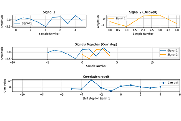
First Method: Time Domain Cross-Correlation
In signal processing, cross–correlation is a measure of similarity of two series as a function of the displacement of one relative to the other. This is also known as a sliding dot product or sliding inner product. It is commonly used for searching a long signal for a shorter, known feature [Wikipedia].
%% Time domain corr
% Time domain in-phase signal
bbSignal = I1 + Q1; %Only in-phase part also enough
tic; %Time measurement begin
% PRN zero padding for correlation
prn = [zeros(1,length(bbSignal)-length(prn)) prn];
[phi_w,mlag]=xcorr(bbSignal,prn);
[val_corr, ind_corr] = max(phi_w);
toc; %Time measurement end
fprintf("\tTime domain correlation running period...\n")
It is a time-domain process. The values in the arrays multiplying each by each after every step of time-shifting one of the arrays. Above, I used “zero-padding”, but you do not have to do it, ‘xcorr’ function is doing what it needs. However, if ‘xcorr’ does it automatically, the place of zeros are located at the beginning of the PRN instead of at the end (manually I did), it will affect the result, you will need an extra subtraction. To get rid of this extra process, I added zeros manually.
Second Method: Frequency Domain Multiplication
The second method based on frequency domain conversion and multiplication. Regarding to the theory indicated in the reference above, cross-correlation in time domain and multiplication in frequency domain produce the same result.
%% FFT of BB signal
% FFT of baseband signal
IQfreqDom = fft(I1 + 1i*Q1);

%% FFT multiplication and IFFT
% FFT multiplication of PRN and received signal at baseband
% Time domain correlation alternative
tic; %Time measurement begin
convCodeIQ1 = IQfreqDom .* conj(fft(prn, length(IQfreqDom)));
%I indicated a length value for fft function, because it is a
%point-by-point multiplication and their length have to be identical

results = abs(ifft(convCodeIQ1));
[val_fft, ind_fft] = max(results);
toc; %Time measurement end
fprintf("\tFFT and IFFT running period...\n")
As claimed that, this method is faster than the correlation for longer arrays. Longer arrays, more time difference. Let’s check it.
Result
The output…
Elapsed time is 0.052317 seconds.
FFT and IFFT running period...

Elapsed time is 0.155647 seconds.
Time domain correlation running period...
As you can see, it is really faster. However, let’s check their values, it is more important…

>> ind_corr

ind_corr =

      604024

>> ind_fft

ind_fft =

      604024
>> val_corr
val_corr =
2.8157e+04
>> val_fft
val_fft =
3.3931e+04Index values are identical, it works! The values at that index may differ, it is related to the “abs” value. You can take the “abs” of the “time-correlated” result also, but you will get the result of the backward counting index.
You can download the signal and PRN data from here.
MATLAB code also here:
Leave a Reply