

We’ll figure out how to estimate a constant based on several noisy measurements of that constant. Assume we have a resistor but don’t know what its resistance is. We use a multimeter to measure its resistance several times, but the measurements are noisy because we have a cheap multimeter. On the basis of our noisy measurements, we want to estimate the resistance. In this case, we want to estimate a constant scalar (can be used for estimating a constant vector also).
To formulate the issue mathematically, assume that x is a constant and y is a k-element noisy measurement vector. How can we determine the constant’s “best” estimate?
We’ll be working with an unlabeled resistor and some noisy data from a multimeter to figure out its resistance.

This single matrix equation may be created by combining these k equations as
![\left[\begin{array}{c}y_{1} \\\vdots \\y_{k}\end{array}\right]=\left[\begin{array}{c}1 \\\vdots \\1\end{array}\right] x+\left[\begin{array}{c}v_{1} \\\vdots \\v_{k}\end{array}\right]](https://unalfaruk.com/wp-content/ql-cache/quicklatex.com-a54336e6dd8ac637f271cfbdbd39630d_l3.png "Rendered by QuickLaTeX.com")
The resistance’s ideal estimate is given[1] as
![\begin{aligned}\hat{x} &=\left(H^{T} H\right)^{-1} H^{T} y \\&=\left(\left[\begin{array}{lll}1 & \cdots & 1\end{array}\right]\left[\begin{array}{c}1 \\\vdots \\1\end{array}\right]\right)^{-1}\left[\begin{array}{lll}1 & \cdots & 1\end{array}\right]\left[\begin{array}{c}y_{1} \\\vdots \\y_{k}\end{array}\right] \\&=\frac{1}{k}\left(y_{1}+\cdots+y_{k}\right)\end{aligned}](https://unalfaruk.com/wp-content/ql-cache/quicklatex.com-b385f6e8d55648571c7109a71cdc0cd2_l3.png "Rendered by QuickLaTeX.com")
We can see that the estimate is just the average of all the measurements.
Let’s carry it out in a coding language. You might need to measure something for an electronics project, and measuring equipment is always directly relevant to noise issues. Although this technique is really basic, it serves as the foundation for more sophisticated ones which I’ll demonstrate later.
Any programming language can be used, however, MATLAB or Python may be preferable since their scientific libraries are easy to use when simulating an environment. In this example, I will produce noise signals in a simulated environment, which needs the use of a library.
However, using the method described above, I will examine two separate sensors. We’ll see how effective it is with accurate and non-accurate sensors.
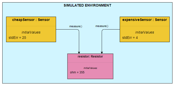
class Resistor:
    def __init__(self,ohm):
        self.ohm = ohm

class Sensor:
    def __init__(self,mean,std):
        self.inputVal = []
        self.outputVal = []
        self.err_std = std
        self.mean = mean

    def measure(self,realVal):
        self.inputVal.append(realVal)
        self.outputVal.append(realVal+np.random.normal(self.mean,self.err_std))

    def meanOfResult(self):
        return np.sum(self.outputVal)/len(self.outputVal)
resistor = Resistor(355)
sensorCheap = Sensor(0,25)
sensorExpensive = Sensor(0,4)A few measurement…
Take 10 measurements and examine the histogram of the findings.
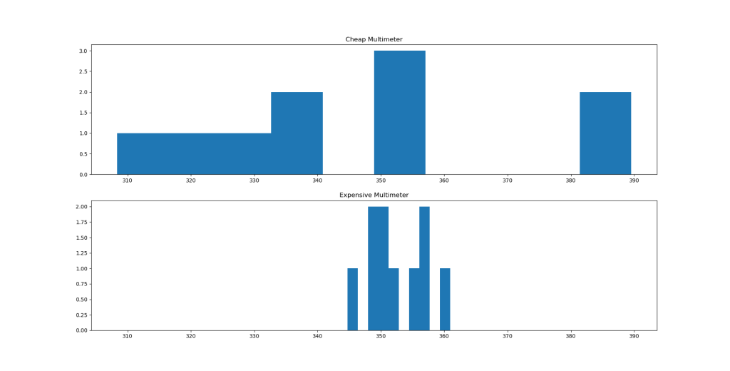
The costly one, as seen above, is close to the real value thanks to to its error characteristics.
What about their estimation results?
| cheap | 346.6066538966017 |
| expensive | 352.1467128829743 |
More measurement…
Take 500 measurements and examine the histogram of the findings.
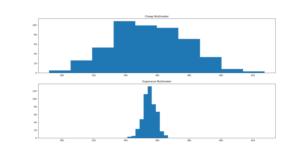
The more expensive one, as seen above, is more accurate thanks to its error characteristics. However, the cheaper option seems to go well.
What about their estimation results with more measurement?
| cheap | 354.769081530342 |
| expensive | 355.12260272431536 |
More measurement, more accuracy even a cheap sensor…
COMPLETE CODE for the SIMULATION ABOVE
[1] Simon, D. (2006). Optimal state estimation: Kalman, H infinity, and nonlinear approaches. John Wiley & Sons. | 3. Least squares estimation
Leave a Reply