

In the last post, we assumed that we had equal confidence in all of our measurements. Assume we have greater confidence in some measurements than others. In this scenario, we must generalize the earlier post’s principles to get a weighted least squares estimate.
A high-end, low-noise multimeter was used for some of the measurements, while an inexpensive multimeter was used for others. We should somehow give the first set of measurements more weight than the other since we have more trust in it. This post discusses that we may actually learn some things from less accurate measurements. Regardless of how inaccurate they may be, measurements should never be dismissed.
The equation below, which is an altered version of the one in the earlier post, demonstrates the weighted estimation of the resistance:
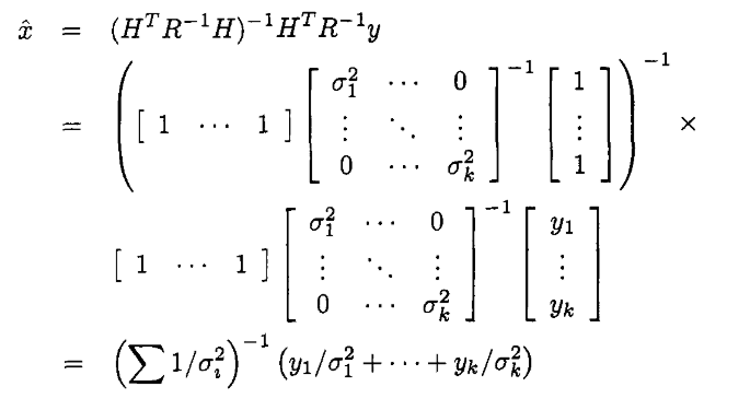
where

Let’s carry it out in a coding language for a simulation. And analyze a few cases.
Case 1: Sensors with the Same Error Characteristics
| SENSOR | DEVIATION |
| Cheap | 4 |
| Expensive | 4 |
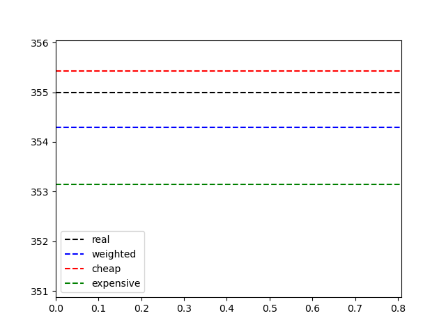
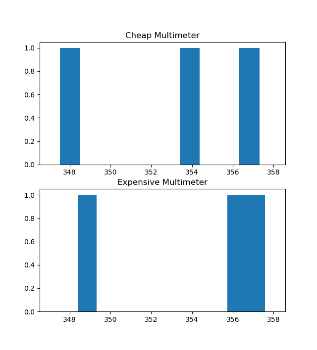
Let’s perform a single measurement to examine the equation (With the single measurement our equation will be clear and easier to follow.)
The resistor has a value of 355 ohm.
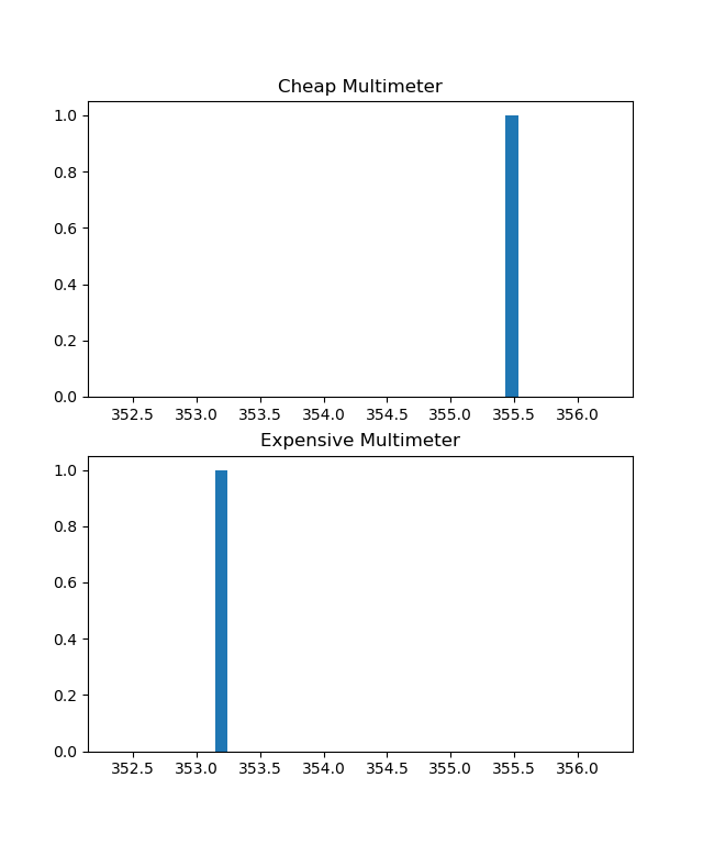
Let’s look at the equations in this case.
The generic equation	:	(1/16+1/16) (355.4/16.0+353.1/16.0)
Weighted measurements	:	0.500*355.432 + 0.500*353.146
Both measurements have the same weight in the outcome, as we can see above. As a result of sensors’ common value of variance.
Let’s take more measurements, but not too many. Let’s say 3.
The generic equation	:(1/16+1/16+1/16+1/16+1/16+1/16) (357.3/16.0+353.4/16.0+347.5/16.0+356.1/16.0+348.4/16.0+357.6/16.0)
Weighted measurements	:0.167*357.304 + 0.167*353.438 + 0.167*347.529 + 0.167*356.142 + 0.167*348.409 + 0.167*357.574
The same weight value applies to all measures, as can be seen above. Because the variance values for both sensors are the same.
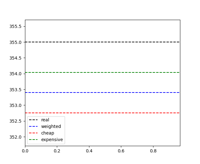
Case 2: Sensors with Different Error Characteristics
This illustration will help you better understand the concept. Due to the various sensor characteristics in this scenario, each measurement will have a different weight value in the final result.
| SENSOR | DEVIATION |
| Cheap | 11 |
| Expensive | 3 |
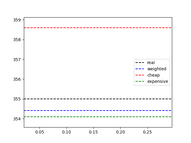
Let’s perform a single measurement to examine the equation again (With the single measurement our equation will be clear and easier to follow.)
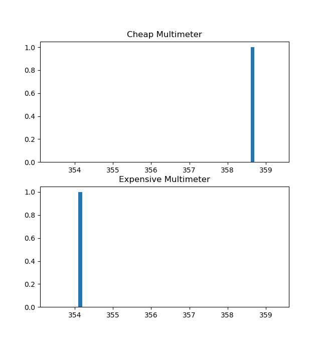
The generic equation	:(1/121+1/9) (358.6/121.0+354.1/9.0)
Weighted measurements	:0.069*358.605 + 0.931*354.094
Please observe the coefficients in the final equation carefully. Can you make out a pattern related to the sensor variance values?
Let’s repeat the case by taking 3 measurements.
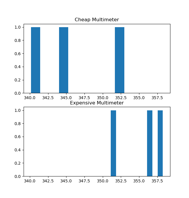
The generic equation	:(1/121+1/121+1/121+1/9+1/9+1/9) (345.0/121.0+353.0/121.0+340.2/121.0+358.2/9.0+351.1/9.0+356.4/9.0)
Weighted measurements	:0.023*344.990 + 0.023*352.967 + 0.023*340.158 + 0.310*358.248 + 0.310*351.115 + 0.310*356.363
Please review the coefficients once again. The sensor variance values and the coefficients are related.
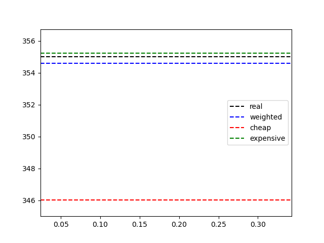
As a result, the relationship between measurement weight and sensor variance is inverse.
[1] Simon, D. (2006). Optimal state estimation: Kalman, H Infinity, and nonlinear approaches. John Wiley & Sons. | 3. Least squares estimation
Leave a Reply